Multitaper

Introduction

The multitaper functions presented here are adapted from the ptmtPH.m script by Peter Huybers (for the calculation of the power spectrum) and from the JD_spectra.m (see also the deshayes_CNRS_IRD_2013_csm5.pdf file for a description of the method).

Plotting the spectrum

The plotting of the spectrum is achieved by using the envtoolkit.spectral.plot_spectra() function. It takes as argument the time series from which to plot the spectra, the time-sampling period (in seconds) and the period at which to plot the error bar. Additional arguments are the spectrum type (variance or energy spectrum) and the number of tapers. Arguments associated with the matplotlib.pyplot.plot() function can be also used. The outputs are the power spectrum, the associated frequency and the error bar.

spec, freq, error = envtoolkit.spectral.plot_spectra(sst, deltat,
                                                  ferror, spec_type='variance',
                                                  nbandw=3, color='k')

Determining the slope

It might be interesting to dermine the slope of a power spectrum. This is achieved by using the envtoolkit.spectral.plot_slope() function. It takes as an argument the spectrum and frequency outputs of the envtoolkit.spectral.plot_spectra() function. It may also takes as argument the first and/or last frequency on which to compute the slope (if not set, the slope is computed over the entire frequency range). It may also take as argument the vertical offset of the slope lines (in order to improve readability of the figure) and arguments which are associated with the matplotlib.pyplot.plot() function. It returns the value of the slope.

slope = envtoolkit.spectral.plot_slope(spec, freq, fmin=1e-2,
                                    fmax=1, offy=2,
                                    color='FireBrick', linestyle='--')

Overlying reference slopes

In a figure, the user may want to plot one or several reference slopes, in order to highlight the value of the slope associated with the the power spectrum. Thisis achieved by using the envtoolkit.spectral.plot_slope() function. It takes as argument the lower and upper frequency value on which to plot the slope, the slope intercept and the value of the slope. It also handles additional arguments associated with the matplotlib.pyplot.plot() function.

envtoolkit.spectral.plot_ref_slope(fmin_slope, fmax_slope,
                                yinter_slope, slope=-3,
                                color='k', linestyle='--')

Example

# Example on the use of multi-taper spectral analysis

import numpy as np
import pylab as plt
import envtoolkit.spectral

# Loading SST data
filein = np.load('sst_taper.npz')
sst = filein['sst']

# defining the delta t and the localisation of
# the error bar
deltat = 30*24*60*60
ferror = 1e-2

fmin_slope = 1e-2
fmax_slope = 1e-1
yinter_slope = 1e-1

fig = plt.figure()
ax = plt.gca()

# plotting the power spectrum (variance type)
spectrum, freq, error = \
        envtoolkit.spectral.plot_spectra(sst, deltat, ferror,
                                      spec_type='variance',
                                      nbandw=3, color='k')

# ploting the slope, computed from freq[0] to 1
# offy = 2, we move the slope by two grid cells on the vertical
slope1 = envtoolkit.spectral.plot_slope(spectrum, freq, fmax=1,
                                     offy=2, color='FireBrick', linestyle='--')

# plotting the slope, computed from 1 to freq[-1]
# offy = 2, we move the slope by two grid cells on the vertical
slope2 = envtoolkit.spectral.plot_slope(spectrum, freq,
                                     fmin=1, offy=2,
                                     color='DarkOrange', linestyle='--')

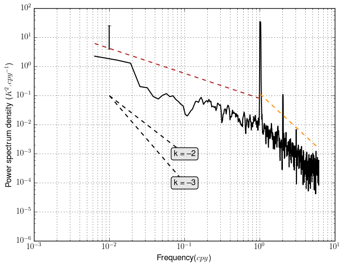
# plotting reference slope (slope = -2)
envtoolkit.spectral.plot_ref_slope(fmin_slope, fmax_slope,
                                yinter_slope, slope=-2,
                                color='k', linestyle='--')

# plotting reference slope (slope = -3)
envtoolkit.spectral.plot_ref_slope(fmin_slope, fmax_slope,
                                yinter_slope, slope=-3,
                                color='k', linestyle='--')

# Defining the x and y labels
ax.set_ylabel("Power spectrum density ($K^2.cpy^{-1}$)")
ax.set_xlabel("Frequency($cpy$)")

# setting the ylim
plt.ylim(1e-6, 1e2)

plt.savefig('figure_mtaper.png', bbox_inches='tight')

print slope1, slope2