Climatologies
Daily time scales
Daily climatologies are computed by using the
envtoolkit.ts.compute_daily_clim() function:
import envtoolkit.ts
clim = envtoolkit.ts.compute_daily_clim(data, date, smooth=True, nharm=2)
The data variable is the variable from which the climatology is extracted. It can be of any dimension, but the climatology is computed on the first dimension (which should be time). The date variable is the date associated with the data, with a format YYYYMMDD (YYYY=year, MM=month, DD=day). It must have the same length as the first dimension of data.
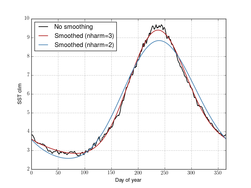
The smooth arguments defines whether the seasonal cycle should be smoothed out. If set to True, a filtering is applied through fft computation. The nharm argument is the number of harmonics to retain in the fft calculation. For instance, a value of 2 means to use the annual and semi-annual harmonics only.
Anomalies are computed by using the function envtoolkit.ts.compute_daily_anom()
anom = envtoolkit.ts.compute_daily_anom(data, date, clim)
The two first arguments are the same as for the
envtoolkit.ts.compute_daily_clim() function, while the last one is the
climatology that was computed on the previous step.
Monthly time scales
The computations of monthly seasonal cycles and monthly anomalies relative to these seasonal cycles are very similar to the computations for daily time scales.
import envtoolkit.ts
clim = envtoolkit.ts.compute_monthly_clim(data, date)
anom = envtoolkit.ts.compute_monthly_anom(data, date, clim)
In the envtoolkit.ts.compute_monthly_clim() function, data is the
data array, the seasonal cycle of which to extract (with time as the
first dimension). date is a date vector, with a format YYYYMM (YYYY=year,
MM=month). Note that contrary to the daily counterpart, there
is no smoothing possible here.
Example
# Example for daily/montly climatologies
import envtoolkit.ts, envtoolkit.nc
import numpy as np
import pylab as plt
from netCDF4 import Dataset
from netcdftime import utime
# defining some plot options
plt.matplotlib.rcParams['lines.linewidth'] = 1
prop = plt.matplotlib.font_manager.FontProperties(size=9)
# recovering sst from a netcdf fime
# converting daily time into dates
filein = Dataset("ts_sst.nc", "r")
data = filein.variables["sst"][:, 0, 0]
time = filein.variables["time"]
cdftime = utime(time.units)
time = time[:]
date = cdftime.num2date(time)
filein.close()
# ============================= processing daily time scales
# converting dates into yyyymmdd formats
# yyyy = years, mm = months, dd = days
yyyymmdd = envtoolkit.ts.make_yymmdd(date)
# daily clim with two harmonics retained (default)
dclim = envtoolkit.ts.compute_daily_clim(data, yyyymmdd)
# daily clim no smoothing
dclim_nosmth = envtoolkit.ts.compute_daily_clim(data, yyyymmdd, smooth=False)
# daily clim threee harmonics retained
dclim_nh3 = envtoolkit.ts.compute_daily_clim(data, yyyymmdd, nharm=3)
# daily anom
danom = envtoolkit.ts.compute_daily_anom(data, yyyymmdd, dclim)
# defining daily xticks and xticklabels
datestr = np.array([d.strftime("%Y-%m-%d") for d in date])
days = np.array([d.day for d in date])
month = np.array([d.month for d in date])
iticks = np.nonzero((days == 1) & (month == 1))[0][::2]
# ============================ processing monthly time scales
# calculating monthly means from daily values
yyyymm, datam = envtoolkit.ts.make_monthly_means(data, yyyymmdd)
yyyymm, timem = envtoolkit.ts.make_monthly_means(time, yyyymmdd)
# monthly clim and anoms
dclimm = envtoolkit.ts.compute_monthly_clim(datam, yyyymm)
danomm = envtoolkit.ts.compute_monthly_anom(datam, yyyymm, dclimm)
# extracting the date from the monthly time values
# defining the monthly xticks and xticklabels
datem = cdftime.num2date(timem)
datestrm = np.array([d.strftime("%Y-%m-%d") for d in datem])
monthm = np.array([d.month for d in datem])
iticksm = np.nonzero(monthm == 1)[0][::2]
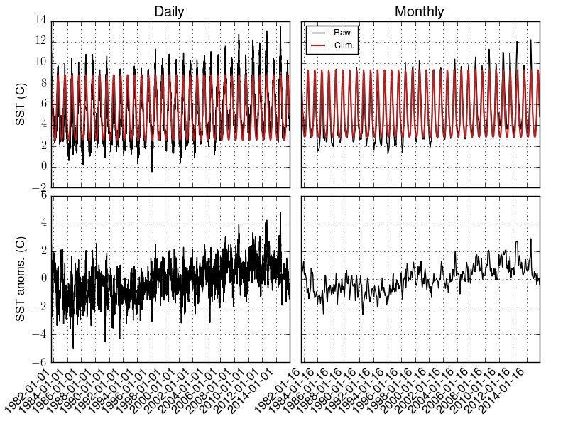
# plotting
plt.figure()
plt.subplots_adjust(hspace=0.05, left=0.09, right=0.95, bottom=0.15, top=0.95, wspace=0.05)
ax1 = plt.subplot(2, 2, 1)
plt.title("Daily")
plt.plot(time, data, label="Raw")
plt.plot(time, data-danom, label="Clim.", linewidth=1.5)
plt.setp(ax1.get_xticklabels(), visible=False)
plt.grid(True)
plt.ylabel('SST (C)')
ax3 = plt.subplot(2, 2, 3, sharex=ax1)
plt.plot(time, danom, label="Anom.")
plt.grid(True)
ax3.set_xlim(time.min(), time.max())
ax3.set_xticks(time[iticks])
ax3.set_xticklabels(datestr[iticks], rotation=45, ha="right")
plt.ylabel('SST anoms. (C)')
ax2 = plt.subplot(2, 2, 2, sharey=ax1)
plt.title("Monthly")
plt.plot(timem, datam, label="Raw")
plt.plot(timem, datam-danomm, label="Clim.", linewidth=1.5)
ax2.legend(loc=0, prop=prop)
plt.setp(ax2.get_xticklabels(), visible=False)
plt.setp(ax2.get_yticklabels(), visible=False)
plt.grid(True)
ax4 = plt.subplot(2, 2, 4, sharex=ax2, sharey=ax3)
plt.plot(timem, danomm, label="Anom.")
plt.grid(True)
ax4.set_xlim(timem.min(), timem.max())
ax4.set_xticks(timem[iticksm])
ax4.set_xticklabels(datestrm[iticksm], rotation=45, ha="right")
plt.setp(ax4.get_yticklabels(), visible=False)
plt.savefig("figure_climato.png")
plt.matplotlib.rcParams['lines.linewidth'] = 1.5
plt.figure()
plt.plot(dclim_nosmth, label="No smoothing")
plt.plot(dclim_nh3, label="Smoothed (nharm=3)")
plt.plot(dclim, label="Smoothed (nharm=2)")
plt.xlim(0, len(dclim)-1)
plt.grid(True)
plt.xlabel("Day of year")
plt.ylabel("SST clim")
plt.legend(loc=0)
plt.savefig("figure_climato_2.png")